
Introduction
Understanding Neighborhood Change
Households move for a variety of reasons. Rossi's (1955) work established a key framework for household moves and the motivations behind them. Some are beneficial, like relocating for a new career opportunity or being closer to family for support, while others are not, like evictions or unaffordable housing costs. The latter reasons are of concern, particularly for households experiencing housing instability. Over time, these collective movements change the resident composition of neighborhoods, the overall topic of interest for this inquiry.
One well-researched aspect of neighborhood change is the phenomenon of gentrification. Originally coined by Ruth Glass (1964) as the socioeconomic upgrading of neighborhoods resulting in the displacement of households with lower incomes. Gentrification is a prime example of how urban redevelopment impacts physical and social structures that, in turn, exacerbate household instability and affect place attachments. Disruptions of emotional bonds between people and place (e.g., place attachments) have far-reaching implications, not just for individuals but for collective wellbeing (Altman & Low, 1992). Developing place attachments comes from consistent daily experiences of place, the human-environment relationship, which is how meaning is derived (Tuan, 1979). Limiting stark disruptions to households in turn nurtures the potential for place attachment (Song & Levine, 2024), which has been found to be meaningful for youth and their long-term outcomes (Anastasio & Leventhal, 2023).
While gentrification has become a common concept in academic and policy literature, little agreement exists on its definition and measurement, because depending on the specific socioeconomic variables (e.g., education, income, housing rents/value, race/ethnicity) used can yield different spatial results (Brown-Saracino, 2017; Finio, 2022). Regardless, gentrification research tends to focus on triggers manifesting in places and the ensuing socioeconomic and demographic aftermaths experienced by, in many cases, historically disadvantaged residents.
Together, gentrification and economic mobility research have produced significant insights on vulnerability and opportunities faced by renter and owner households (Chetty & Hendren, 2018; DeLuca et al., 2019; Desmond & Perkins, 2016; Freeman, 2005; Hepburn et al., 2024). However, up until the past decade, gentrification largely produced a singular focus on the displacement of vulnerable households from qualifying neighborhoods (Galster & Peacock, 1986; Glaeser et al., 2018; Marcuse, 1985; Rucks-Ahidiana, 2021; Smith, 1979; Zuk et al., 2018). Fortunately, recent research has turned its attention to the receiving neighborhoods which have received less attention (DeLuca et al., 2019; Freeman et al., 2024; Hepburn et al., 2024). Vulnerable households can experience displacement from neighborhoods not defined as gentrifying, yet this instability largely goes unnoticed (Desmond & Shollenberger, 2015; Evans, 2021). Exploring household movement more broadly, irrespective of the process of gentrification, can provide further insight into how neighborhoods change, and target solutions to enhance economic mobility opportunities (Hepburn et al., 2024).
Identifying receiving neighborhoods: a timing challenge
Household economic mobility implies knowledge of where households are located or the origin and destination of individuals moving in the context of the neighborhood’s socioeconomic characteristics (Chetty & Hendren, 2018). However, more work is needed to understand the neighborhood change as a function of household movement. Vulnerable households often move to new neighborhoods, but a systematic quantification of these spatial patterns has been impractical or significantly delayed due to existing data resources. Past research was left to assessing neighborhood change from an archival perspective (Delmelle, 2017). Research points to this timing gap by finding ways with existing administrative data to identify the receiving neighborhoods in order to meet vulnerable households where they are in a timelier manner (Freeman et al., 2025).
A key goal of this project is to establish a more complete accounting of household movement, referred to as “household churn.” Specifically, I focus on the ability to identify receiving neighborhoods. This paper seeks to better understand place dynamics using voter records as a novel data source to explore the relationship between incoming household churn and changes in income, a facet of economic mobility, in the city of Denver, by asking the following explicitly spatial questions:
What are the patterns of neighborhood-level household churn in Denver? How are the identified patterns of churn related to and affected by socioeconomic factors associated with economic mobility?
Methods
Household churn as a quantifiable concept
All human migration has an origin (departing location) and a destination (new location). Collectively, these leaving and incoming movements in an urban neighborhood are what I refer to as “household churn.” Quantifying this activity enables thorough exploration of the relationship between household movement and economic opportunity in a local context. For this study, I constructed a proxy variable capturing the movement of new households to places (e.g., census tracts). While departing households constitute the other half of the household churn dynamic, new households have great influence on socioeconomic changes in neighborhoods. For purposes of this analysis, the direction of the relationship establishes incoming rates of household churn as a function of income changes.
Study area
Conducting this work in Denver was made possible by the public availability of data to construct the incoming household churn variable. Census 2010 tracts are the geographical unit of analysis to align with the years of data used in the analysis. Census tracts have been widely used as a proxy for neighborhoods (Finio, 2022). The City of Denver uses census tracts to construct their statistical neighborhoods, which are used as an overlay for ease of reporting and visualizing results (Geospatial Denver, 2025).
Data processing
The questions for this study require moving beyond traditional neighborhood change assessments tied to aggregate socioeconomic indicators, such as the American Community Survey (ACS). However, data availability to conduct such skip tracing analysis to identify receiving neighborhoods has generally been limited beyond sampling from national surveys, specific social programs, or access to highly restricted tax records (Chetty & Hendren, 2018; DeLuca et al., 2019; Freeman et al., 2024). Fortunately, robust longitudinal household location information exists through Colorado’s Secretary of State’s voter records (Elections Division, 2026). These data, in conjunction with assessor records and ACS indicators, will serve as the core data utilized in the analysis for this work.
Voter addresses were matched to assessor parcel addresses (with fuzzy logic), and then spatially joined to census tracts. This nesting of data sources (voter households – parcels – tracts) enables the aggregation of household moves over time by tract. This skip tracing analysis provides the foundation for quantifying household churn in spatially and temporally discrete ways. Each churning household was tagged based on the “departing” address and the “receiving” address. Finally, I constructed a longitudinal origin-destination matrix to capture the two aspects of household churn (departing and incoming) and built the dependent variable, incoming household churn. Conversely, by tying the data sources to census tracts enabled construction of an economic opportunity proxy independent variable from the ACS (Ruggles, 2025). I hypothesize that there is an association between changes in median household income and with incoming household churn (Chetty & Hendren, 2018; Freeman, 2005). Figure 1 captures the workflow of variable development.
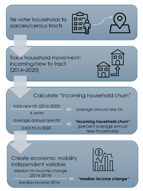
Figure 1. The workflow of variable development. Obtained from author.
Assessing normalcy of "incoming household churn"
Before moving to the statistical analysis, it was necessary to explore and characterize the dependent variable, incoming household churn. RStudio was used for the following assessment. The measures of central tendency, median = 0.30 and mean = 0.29, indicate a compact interquartile range of 0.25 to 0.33. With a minimum of 0.15 and a maximum of 0.43, the full range indicates at least some level of incoming household churn, up to almost half being new, on average. When plotting the variable in a histogram (Figure 2) it visually exhibited sufficient normalcy. Skewness was estimated at -0.33, a left-tail negative skew. Shapiro-Wilk normality test results were W = 0.98123 with a p-value of 0.04572. While these outputs do not provide an indication of strong statistical normalcy, the data distribution has a normal enough pattern to enable parametric analysis.
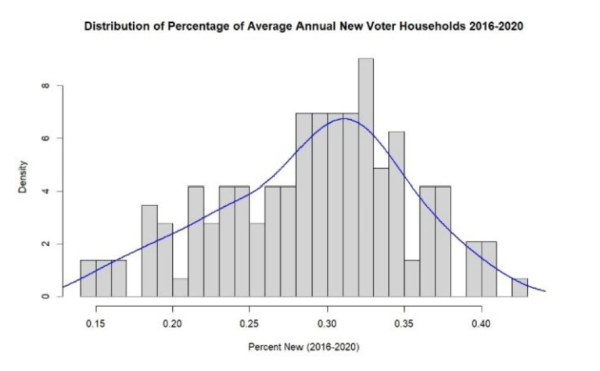
Figure 2. Distribution of percentage of annual new voter households from 2016-2020. Obtained from author.
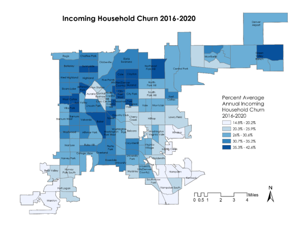
Figure 3. Spatial distribution of incoming household churn. Obtained from author.
Analytic approach
This spatial inquiry relies on parsimonious analytic methods. Anselin Local Moran’s I and Getis Ord Gi* (run in ArcGIS Pro) identifies clusters/outliers and hot and cold spots patterns, of the percentage of average annual incoming household churn (2016-2020). Utilizing both methods together offers an approach to examine spatial autocorrelation. Anselin Local Moran’s I identifies regions where there is negative spatial autocorrelation (How Cluster and Outlier Analysis (Anselin Local Moran’s I) Works—ArcGIS Pro | Documentation, n.d.). Both analyses conceptualize spatial relationships and applied false discovery rate (FDR) using an inverse distance model to ensure a higher level of confidence.
Lee’s L bivariate spatial association (ArcGIS Pro) illustrates the tract-level spatial patterns of the correlations between incoming household churn and median income change (Bivariate Spatial Association (Lee’s L) (Spatial Statistics)—ArcGIS Pro | Documentation, n.d.). The tool uses K nearest neighbors (eight) for selecting data points considered in the analysis, which results in an adaptive distance model that uses different locations (driven by the proximity of the eight nearest neighbors).
OLS Linear Regression (global) (RStudio) serves to identify the extent to which change in median income affects incoming household churn.
Visualizations
All results were mapped using the geographic information system (GIS) software ArcGIS Pro (Esri Inc., 2025). The census tract shapefile used to visualize results was obtained from the National Historical Geographic Information System (NHGIS) (Minnesota Population Center, 2025). The neighborhood shapefile used for neighborhood labeling on the maps was obtained from the City and County of Denver Open Data Catalog (Geospatial Denver, 2025).
Results
Spatial autocorrelation: clustering/outliers and hot/cold spots
Results from Anselin Local Moran’s I and Getis Ord Gi* testing for spatial autocorrelation of incoming household churn, (Figures 4 and 5), indicate similar spatial patterns. The clustering/outliers result in Figure 4 shows high clustering throughout the center and northwest area of the city, and in the city core. The city core and areas to the east and southeast indicate negative spatial autocorrelation. Areas to the far southeast, east central, and far southwest have statistically significant low levels of churn. The hot/cold spots result Figure 5 shows statistically significant hot spots of incoming household churn from Cherry Creek across the entirety of the city center and to the west and north. Areas to the far southeast and further southwest are statistically significant cold spots of incoming household churn, representing areas of high residential stability.

Figure 4. Cluster & Outliers (Anselin Local Moran's I) Incoming Household Churn. Obtained from author.
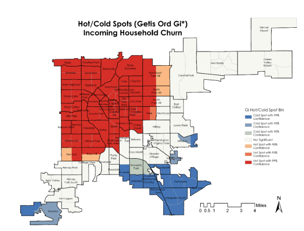
Figure 5. Hot/Cold Spots (Gettis Ord Gi*) Incoming Household Churn. Obtained from author.
Correlation: Bivariate Spatial Association (Lee's L)
Figure 6 presents a map of the bivariate spatial association (Lee’s L) of incoming household churn and median household income change. Areas of high-high association are in the west, north, northeast and south central from the central city. Low-low association areas, areas where both churn and income change are low, are in the southwest, southeast and east-central parts of the city. Lee’s L statistic (Table 1) value of 0.17 is statistically significant and indicates a positive but weak bivariate spatial association. This contrasts with Pearson’s R measure of 0.30, a global measure that does not capture spatial autocorrelation.
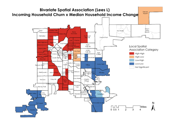
Figure 6. Bivariate Spatial Association (Lee's L) Incoming Household Churn x Median Household Income Change.
| Summary of Bivariate Spatial Association (Lee's L) | |
|---|---|
| Global Lee's L | 0.1743 |
| Global P-value | 0.0020 |
| Spatial Smoothing Scalar (per_ann_new_churn1620) | 0.5341 |
| Spatial Smoothing Scalar (per_medinc_chg) | 0.1530 |
| Pearson Correlation (raw) | 0.3031 |
| Pearson Correlation (neighborhood averages) | 0.6089 |
Table 1. Summary of Bivariate Spatial Association (Lee’s L). Obtained from author.
Regression: OLS Linear Model
Results from the global OLS regression assessing incoming household churn as a function of change in median income indicate a statistically significant but small (0.09) effect. Incoming household churn increased an average of 0.09 percent with every percent increase in change in median household income. The model explains approximately nine percent of the variation in incoming household churn (r2 = 0.088).

Figure 7. Results from the global OLS regression assessing incoming household churn as a function of change in median income. Obtained from author.
Limitations
These results should be interpreted with careful consideration of the limitations.
While Colorado has high rates of voter registration, utilizing voter records does not capture all household movement as it does not include households without registered voters. Consequently, the results herein underestimate the incoming household churn.
Additionally, modeling in this study was performed at the census tract geographic unit of analysis, and so results cannot be extended to smaller or larger geographic units (doing so would commit an ecological fallacy). In addition, results could change if the study area is expanded to the metropolitan region.
As a global model, the base regression modeling is unable to isolate spatial autocorrelation and leaves the potential for additional confounding variables to exist. For instance, because I measured incoming household churn, the observed clustering could be influenced by areas of the city where new development occurred, which was not measured. If data can be collected at sufficiently high enough resolution to add some statistical power, future work could address spatial autocorrelation and examine the spatial structure of patterns by using a geographically weighted regression or spatial autoregression models.
While economic mobility research has established the connection between household moves and income outcomes, other factors can influence a household’s decision to move. For instance, testing real estate investor activity could add to future work to assess the effect of economic externalities on household movement.
Establishing the direction of causality is a common problem in longitudinal urban studies. It is not clear how household churn affects changing neighborhood characteristics, and so future work could consider this relation as well as temporal lag, through difference-in-difference modeling.
Unfortunately, the available data did not enable alignment of the study periods, which is an additional limitation. Incoming household churn data were aggregated for 2016-2020, while the median income change represents the change between two five-year ACS periods, 2010-2014 and 2015-2019. Examining changes across multiple geographies could better specify and improve the model in future efforts.
Conclusion
Discussion and future research questions
Drivers of individual households’ movement are diverse and complicated. Incoming household churn, a proxy measure created from voter records, demonstrated strong positive spatial autocorrelation (clustering) in large sections of the city. These spatial patterns are consistent with local patterns of development and socioeconomic changes in the city. Development activity and proximity to central amenities attract new households, while older, more stable and quiet areas are more distance. Low and high local spatial correlation (with change in median income) also exhibit locally intuitive patterns, such as glimpses of Denver’s “inverted L,” along the western neighborhoods and turning east along the northern boundary, areas known to experience gentrification (Social Equity & Innovation, 2023). Validation from these results and Freeman et al.'s (2025) validation of using voter records as a novel data source together establish confidence in the utilization of voter data as a proxy of household churn in future analysis in Colorado.
Comparing the spatial autocorrelation results and the bivariate spatial association revealed potential pathways for additional study of hot spots in household churn, yet I observed no association with household income changes. These areas could be particularly important as markers of vulnerable household churn but require future analysis to understand the drivers of this household instability, such as evictions, and inform the development of supportive solutions. By including the entire city in this analysis, vulnerability in receiving neighborhoods, irrespective of gentrification, is made visible and contributes to advancing ways to fill this spatial gap in information (Desmond & Shollenberger, 2015; Evans, 2021; Freeman et al., 2024). Insight into household movement in and among all economically vulnerable areas can provide guidance for cities on where to directly engage with residents to better understand their needs, and can target critical stabilization support (DeLuca et al., 2019). Specifically, we can begin to explore the relationship between experiences of displacement and place attachment and the implications for broader community wellbeing, especially for the next generation (Altman & Low, 1992; Song & Levine, 2024).
Fortunately, the spatial patterns depicted from these analyses demonstrate that voter records can serve as a viable and effective data source to build proxy household churn measures across large geographic areas. The benefit of using timely, discrete household-level administrative data expands the ability to be geographically inclusive and therefore inclusive of all types of social processes (Delmelle, 2016). Opening the lens to encompass all forms of household churn will enable more robust research to assess displacement and its spatial patterns more broadly in the context of neighborhood change. Leveraging this methodology to provide timely information on household churn can also aid in the evaluation and crafting of planning and fiscal policies and public investment decision-making to mitigate unintended consequences such as displacement (Zuk et al., 2018).
Overall, these results help pave the way for future analysis using voter data to better understand the degree of affect socioeconomic and other factors have on household churn (or vice versa) across the seven-county Denver region. This work serves as a proof of concept using voter records as a novel data source. I seek to contribute to the expanding literature on receiving neighborhoods and place attachment by building off this baseline work by asking a new question: Where is household churn the most concerning for economically vulnerable households in metro Denver?
Jennifer Newcomer is a PhD student in the College of Architecture and Planning (PhD Geography, Planning, and Design).